The ultrasound range sensor I’m using has a minimum range of about 16cm, but I thought it would be interesting for my robot to sense objects more closely than that. Sharp have a range of three Infrared Range sensors that are very popular and fairly easy to interface to a Raspberry Pi. I’ve chosen the GP2D120 because it’s got a supported range of 4cm to 30cm.
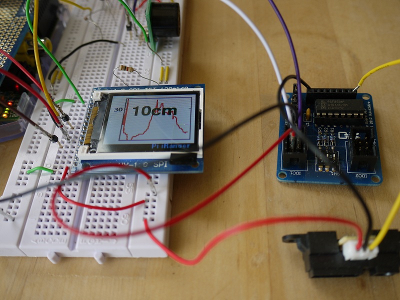
My Raspberry Pi connected to the Quick2Wire I2C ADC and a Sharp IR Ranger
Analogue to digital
Unlike the Ultrasound sensor, you cannot just read the value over I2C because the Sharp rangers output a voltage between 0.29v and 2.97v which is a function of the distance sensed. The Raspberry Pi doesn’t have a builtin analogue input, so I’ve used the PCF8591 I2C Analogue to Digital Converter (ADC) chip, which comes in a very neat breakout kit from Quick2Wire (other ADCs are available), which works just fine on the same I2C bus as the Ultrasound sensor.
Reading values using Python from the ADC is easy enough using Python’s I2C support, assuming you’ve connected the ADc’s channel 0 to something then like this will read the value sensed and display it converted into volts:
pi@raspberrypi ~ $ sudo python
Python 2.7.3 (default, Jan 13 2013, 11:20:46)
[GCC 4.6.3] on linux2
Type "help", "copyright", "credits" or "license" for more information.
>>> import smbus
>>> i2c = smbus.SMBus(1)
>>> print 3.3 / 255.0 * i2c.read_byte(0x48)
Sharp IR Ranger
According to its datasheet, the GP2D120 takes up to 52.9ms (38.3ms±9.6ms measurement + max 5ms for output) between range measurements, or 18.9Hz.
That’s slightly faster than the ultrasound sensor and way more than my ADC’s 200Khz sampling rate, so we should be good to run them from the same timing loop. For now, I’m just messing about with the sensors and processing code, but it should easily slot into my robot’s control loop that runs at slightly less than 10Hz, especially if I leave the ultrasound sensor pinging whilst the rest of the loop does its thing.
As well as its rated minimum, typical and maximum values, the Sharp 2D120’s data sheet includes some graphs of its output in volts against the distance it’s sensed of a reflective object. Between its minimum (4cm) and maximum (30cm) specified range, the sensed voltage is proportional to the reciprocal of the distance. This looks like this:
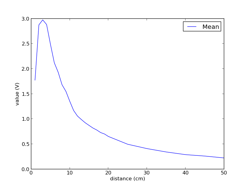
Infrared measured voltage at measured distances
I used the same script to capture calibration data as I used for the ultrasound sensor, looking at the range of 10 readings captured at maximum rate for each measured distance from the sensor. I don’t have a calibrated photographic white or grey sheet of paper, so I just used a large hard-backed book with a white cover that reflected plenty of infra-red light.
You’ll notice that below the minimum rated range of the sensor, the graph shows the sensed value decreasing again. There’s nothing we can do about that, so we just have to ignore it and record that we can’t tell the difference between an object at 1cm and an object at 7cm.
I thought it might be interesting to consider resolution, accuracy and precision of this set up. The ADC I’m using is only 8 bit, so it can report just 255 different values over its active range of 0 to 3.3v, which gives us a resolution of 0.0129v. The ADC samples at 200khz, which is greater than twice the output rate of the IR sensor, so we can be confident we shouldn’t experience sample aliasing.
I measured the active range of my IR sensor to be a bit better than that specified in the datasheet, 2.97v at ~3cm to 0.29v at ~40cm which is 81.2% of the range of the ADC, so we lose a bit of its sampling resolution but it’s close enough for me.
The IR range sensor doesn’t have the same internal calibration as the ultrasound’s sensor, so I thought it might be interesting to graph the minimum and maximum values as well as the mean to illustrate the variance.
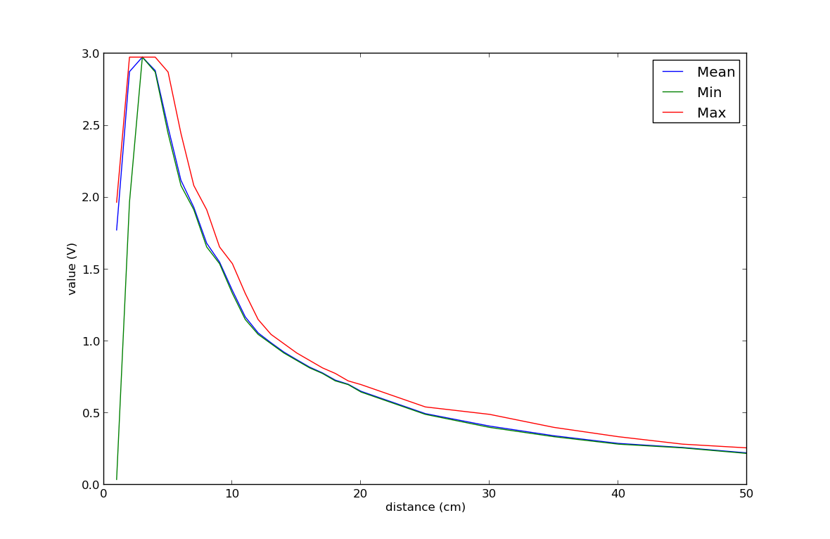
IR min max and mean measurements
Linearising the values from the GP2D120
The key difference between using the IR and Ultrasound sensors is that we need to process the number reported by the IR sensor before we obtain a measurement of distance. Looking at the graphs above, we can see that it isn’t a linear relationship, so fitting a function to that curve will take us a couple of steps.
Now, the datasheet for the sensor helpfully includes a footnote on the last page containing a formula that transforms the values to something much closer to a linear relationship between voltage and distance, but at the cost of introducing an intermediate unit of measurement. My measurements are close enough to those graphed in the datasheet, so that this formula will be an excellent place to start:
linearX = 1 / (d + 0.42)
Linear Regression is a good way to fit a function to this new curve of the form y = mx + c, but I thought I’d see how close I could get just by looking at the values from graphing that function applied to my measurements, included below in blue. Assuming the linear graph passes close enough through the origin, then I went for y = 15.69x, which looks like this green line:
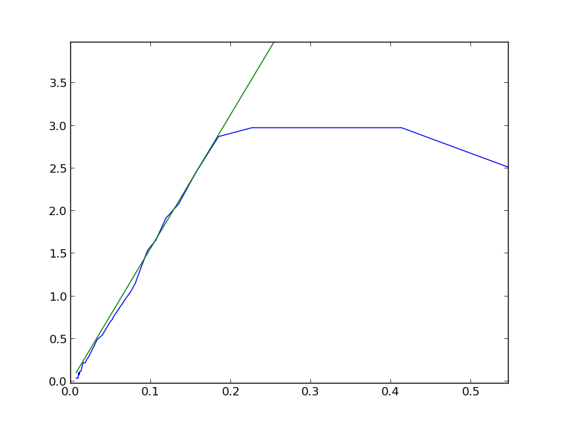
Linearised measured distances in blue and a fitted linear function in green
It’s not a bad fit and it’s close enough for the active area for the graph. So, to bring the equations together we get:
voltage = 15.69 * (1 / distance + 0.42)
or solving it for distance:
distance = (1.0 / (voltage / 15.69)) - 0.42

Mean measured values graphed with values calculated from my function
Fitting that final function onto our original measurements shows that we’re close, our function is of the correct form, but we need to tune the two constants to get it closer. There are some interesting ways that we can calculate the correctness of the fit and how we can find better constants programmatically, but this post is already too long so I’ll gloss over that for now and instead just say that:
distance ~= (1.0 / (voltage / 13.15)) - 0.35
Which looks like this, which is a much closer fit:
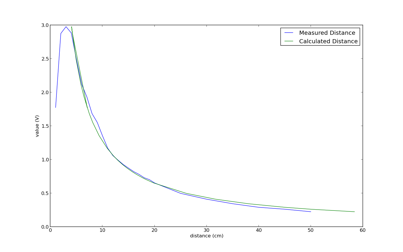
Mean measured values graphed with values calculated from my tuned function
Bringing it all together
IR Ranges from lcdGraph.py
To bring it all together, I’ve swapped in the IR class, adc.py, for the Ultrasound class into the graphing code, lcdGraph.py from before. The classes have similar interfaces so no other changes were required to produce this graph from matplotlib on the Pi itself.
The code
As always, my code’s on github. The scripts are starting to get a bit long to just paste directly into the post, but the most relevant files are:
- adc.py – the class that takes a set of readings from the IR Ranger and converts them into cm
- calibrate.py – the class that does some simple statistics and records many results
- lcdGraph.py – the script that demonstrates how to draw charts headlessly using matplotlib and display them and some text using pygame on a framebuffer. That framebuffer could just as easily be the Pi’s normal HDMI output at 1920×1080