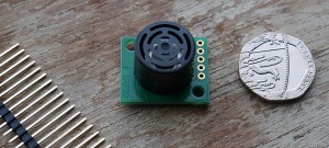
SRF02 sensor. About the size of 20p.
I thought it would be fun if my robot could take measurements of its environment so that it can eventually create maps of its world. My budget won’t quite stretch to a spinning laser beam to create a LIDAR point cloud, so I’m starting out with a ultrasound sensor and an infrared sensor, connected to my Raspberry Pi using its I2C bus. This article explains how I set up the ultrasound sonar sensor.
I’ll gloss over how sonar works to try to keep this article on topic, but Wikipedia has a good diagram of Active Sonar and Devantech have a practical FAQ on using their modules. The important things to know are it has a minimum and maximum effective range, it takes 65ms to take a measurement and it sends out ripples of sound waves in a cone, it’s not a pencil thin straight line.
I2C
This sensor connects to my Raspberry Pi using its I2C bus, so we need to make sure we’ve got that set up and running first. There are any number of detailed guides elsewhere on the internet for how to get that working, but briefly you need to:
- Enable the kernel modules ‘i2c_bcm2708’ and ‘i2c_dev’ by commenting out that line in /etc/modprobe.d/raspi-blacklist.conf
- Reboot, and you should now have device entries for /dev/i2c/0 and /dev/i2c/1
- Once we’ve wired up our sensor, it should show up on address 0x70 when we run:
pi@raspberrypi ~ $ sudo i2cdetect -y 1 0 1 2 3 4 5 6 7 8 9 a b c d e f 00: -- -- -- -- -- -- -- -- -- -- -- -- -- 10: -- -- -- -- -- -- -- -- -- -- -- -- -- -- -- -- 20: -- -- -- -- -- -- -- -- -- -- -- -- -- -- -- -- 30: -- -- -- -- -- -- -- -- -- -- -- -- -- -- -- -- 40: -- -- -- -- -- -- -- -- -- -- -- -- -- -- -- -- 50: -- -- -- -- -- -- -- -- -- -- -- -- -- -- -- -- 60: -- -- -- -- -- -- -- -- -- -- -- -- -- -- -- -- 70: 70 -- -- -- -- -- -- -- - If that works, we can ask the SRF02 for its software version using:
pi@raspberrypi ~ $ sudo i2cget -y 1 0x70 0 b
0x06
Ultrasound
Devantech make an excellent range of ultrasound ranging sensors from their base in Norfolk. I’ve chosen the SRF02 module because it’s cheap, uses a single transducer, is very easy to use over I2C and has an excellent range. Its range is given as 16cm to 6m ±3cm, but in my house its calibration reduces the minimum to about 12cm and I’ve found it to be accurate to 1cm over a range of about 1.5m. I thought for a while that 192cm was its maximum, but it turned out to be just measuring the distance to the ceiling.
The SRF02 runs at 5V, but it seems safe to connect its output directly up to the Raspberry Pi’s 3.3V I2c bus, which saves the headache of having to convert from 3.3v to 5v in both directions on the same two wires. I guess this didn’t blow up my Pi because the I2c pulses are relatively short and infrequent so don’t transmit too much excess energy for the Broadcom chip to dissipate as heat. Health Warning: overloading voltages like this can destroy your Pi, be careful!
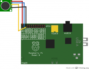
SRF02 Fritzing diagram
It takes 65 milliseconds from issuing the ping command to the result being available, so that’s a maximum of about 15Hz. I don’t know if there are any consequences of running pings so close together, so I’ve been running at about 12.5Hz to be on the safe side.
The datasheet includes a list of all of its commands but for now I’m just using command 81, which sends a ping and returns the result in cm. The sensed range is returned in bytes 2 and 3 of the srf02’s register, with byte 2 being the high byte, so we need to convert that into an integer either by fetching both values individually, multiplying byte 2 by 255 (or rotating it left by 8 bits if you prefer) and then add byte 3, or by treating it as a word and dividing that by 255. In Python, that looks a bit like this:
pi@raspberrypi ~ $ sudo python
Python 2.7.3 (default, Jan 13 2013, 11:20:46)
[GCC 4.6.3] on linux2
Type "help", "copyright", "credits" or "license" for more information.
>>> import smbus
>>> i2c = smbus.SMBus(1)
>>> i2c.write_byte_data(0x70, 0, 81)
>>> print i2c.read_word_data(0x70, 2) / 255
224
>>>
Calibration
I thought it would be interesting to see how repeatable and accurate the sonar’s sensed results are by running some simple statistics and comparing the results in a calibration curve. I threw together a simple python script that takes 10 readings from the sensor, calculates the maximum, minimum and mean (as well as speed, I got a bit carried away), then records that in a text file along with the user’s input for a measured distance to compare it to.
I found the sensed results to be consistently within specifications. I suspect that most of the difference between the mean sensed result and the distance I measured with the steel tape measure is down to experimental error, either with me holding the piece of wood wonky or not lining things up straight, it might also be that I didn’t use a solid enough sonar target.
The upshot to all of this is that I think the results of a single ping can be trusted, we don’t need to smooth the results with a moving window average which means this sensor can be used at or near its maximum sensing speed. Which makes me wonder, if most of its sensitivity is within a 60 degree arc, how quickly could we do a full 180 or 360 degree sweep if we had a stepper motor and turntable.Bringing it all together
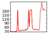
There isn’t much to actually look at so far, so I’ve brought all of the elements together with a slightly more complex python script that takes 4 readings a second and displays the current result on my SPI LCD. Pygame can just about update the LCD’s display quickly enough to keep up with 4Hz. That’s a bit boring though, so I’ve brought in the excellent matplotlib to draw a line chart illustrating the history of distance readings.
Using matplotlib with my framebuffer LCD took me a little while to figure out, both to select the correct backend (Agg) so that it can render without access to GTK or X windows and to display the colours I intended on my LCD as its somehow got its blue and red signals swapped over. I’m sure there must be a better way of transferring the rendered image from matplotlib’s backend to pygame for blitting to the screen, but for now I write a PNG to /tmp in the filesystem and then read it back in again with the other API, before rotating it through 90 degrees and blitting it. Again, ideally I’d like to avoid using pygame to rotate all of the surfaces before they’re blitted by drawing them in the correct orientation in the first place, but this does at least work for now. Drawing the graph takes a couple of seconds, so you’ll see in the video below that the red LED on the back of the sensor pings 8 times over 2 seconds, then pauses for a bit whilst it updates the graph before pinging again. If I intended to use this code for anything vaguely useful, I’d put the chart drawing, sensor pinging and display updating into different threads so they can all just get on with their work without blocking each other, but that would make it harder to read.
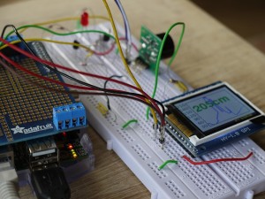
My prototype set-up, showing the Pi, SRF02 and LCD graph display
The code
As always, my code’s on github. The scripts are starting to get a bit long to just paste directly into the post, but the most relevant files are:
- srf02.py – the class that takes a set of readings from the sensor
- calibrate.py – the class that does some simple statistics and records many results
- lcdGraph.py – the script that demonstrates how to draw charts headlessly using matplotlib and display them and some text using pygame on a framebuffer. That framebuffer could just as easily be the Pi’s normal HDMI output at 1920×1080